First try at a linear separator.

I've written the first draft of a linear separator implementation in R, and used it on the famous Old Faithful geyser data set. In the plots below, the x-axis corresponds to the length of an eruption event in seconds, and the y-axis represents the waiting time until the next eruption. Waiting times fall into two general groups: short waiting times after short eruptions, and long waiting times after long eruptions.


My implementation (in its current form) plots the data itself in the scatter plot "Initial State" and then adds a second plot with the data separated into two groups, blue and purple, and the separator shown in orange. (Click the image to enlarge.)

All I know about linear separators I learned in AI class. My code does not use the alpha correction in the update, nor does it find the optimum separator among all possible separators, as Dr. Thrun begins to describe at the 3:40.


My code takes any data set of x,y ordered pairs and subsets it into two by finding centered means of two subsets. It does not matter whether the data set is linearly separable in a formal sense, the algorithm will separate the data into two regardless. 


Without going in to too much detail, the separation process itself happens iteratively in a while loop where y-values of the data points are compared to y-values of the separator line. The initial separator line is the perpendicular bisector of the two points farthest apart from each other. Every point above the line is put in one group, and every point below is put into another group. The algorithm proceeds to draw a new separator as the bisector of the mean x,y position of the two points above and below the previous separator. When the means do not change within a tolerance, the program quits.


In order for this to work, the separator line must not become perfectly vertical or the y-distance between any point and the line would be infinite. 


R has a jitter function that adds a small random number to each and every element of a vector. Here is an example of jitter on a vector x containing 4,5,6:

> x=c(4,5,6)

> x=jitter(x)

> x

[1] 3.996404 5.159189 6.149125

The 4 became 3.996404, 5 became 5.159189, and 6 became 6.149125. Those may be small changes, but I wanted my adjustments to be even smaller.

c=A.1-B.1

if (0 %in% c) {A.1 = A.1 + runif( length(A.1), -.0001, .0001)

               B.1 = B.1 + runif( length(B.1), -.0001, .0001)

                 y = y   + runif(length(y), -.0001, .0001)}

I alter the y-values randomly by an amount greater than -0.0001 and less than 0.0001. When the data is plotted, you can not tell that it was jittered. (Note: This is fine if .0001 is an insignificant amount relative to the values of the data set. It seems obvious now that a second draft of the code should determine what limits of runif would yield an insignificant amount of jitter.)

Shuffling perfectly, using R

The question of how many shuffles it takes to randomize a deck of playing cards has been debated extensively in the mathematical literature. Stanford Professor of Statistics and Mathematics and former professional magician Persi Diaconis is the person perhaps most closely associated with this problem. Along the way, Diaconis and others developed different conceptions of randomness using models of "total variation". Under Diaconis' criteria, it takes 7 good shuffles to randomize a deck. It is easy to obtain a similar number by running simulations in R. I did a little bit of my own work on this problem in graduate school, and I plan to write about it here soon--specifically about what happens when you consider theoretical card decks with many more cards than the standard fifty-two.


However, right now I want to talk about what happens when you do not shuffle the deck randomly. Think about what happens in ordinary card shuffling: you cut the deck in half and interleave the two halves back together by alternately taking small, random numbers of cards from each half. What you do not want to do is take exactly one card, or any fixed number of cards, from each half in alternate succession because that does not randomize the deck, it merely re-orders it. You can predict where each card is after every such shuffle. If you carry out this strict reordering, or "perfect shuffling", a number of times, the deck eventually returns to the same sequence it started with! In the 52-card deck, that number happens to be 8.



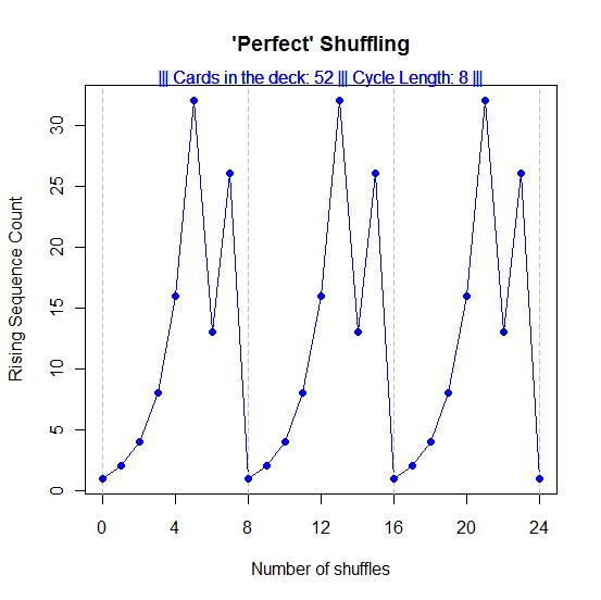The figure above plots the number of "rising sequences" against the number of perfect shuffles. After 5 shuffles on the x-axis, RS=16 on the y-axis. The first blue dot represents the deck in starting position, with x=0 and y=1). I let the cycle run three times so you can see the pattern repeat.


In R, each unique card in the deck may be represented by a number in the sequence 1:52. Starting with a fresh deck is equivalent to starting with the R data vector seq(1:52). Cutting the deck exactly in half gives you two sequences, 1:26 and 27:52. After the first perfect shuffle you have this sequence:

1, 27, 2, 28, 3, 29, 4, 30,....,23, 49, 24, 50, 25, 51, 26, 52

It is easy to see what rising sequences are, and that there are two of them, by looking left-to-right:

1, 27, 2, 28, 3, 29, 4, 30,....,23, 49, 24, 50, 25, 51, 26, 52

And, so it goes, in subsequent shuffles where the number of rising sequences rises and falls until the 8th shuffle at which point you return to the starting sequence with only one rising sequence (henceforth, RS).


Note: In random shuffling, RS reaches an average limit of 26.5. That is to say, once the deck has been shuffled enough times to fully randomize it, RS oscillates between 26 and 27, for eternity. I will talk about this more in a future blog post.


In the meantime, several things intrigued me about the plot above that I obtained from simulating perfect shuffling. For example, I did not anticipate the asymmetry in each cycle. It takes 5 shuffles for the deck to go from RS=1 to RS=16. But the deck goes from RS=26 to RS=1 in one step! That might seem reasonable upon some consideration since 26 is half the deck. You might even guess what the RS=26 sequence looks like, but it is easy enough to pull it out of the program if you cannot. Here is the R output following the 7th perfect shuffle, in standard reading frame, left-to-right, top-to-bottom. (The bracketed number in the first column is the position in the deck of the number just to the right of the bracket.)


[1]   1  3  5  7  9 11 13 15 17 19 21 23 25
[14] 27 29 31 33 35 37 39 41 43 45 47 49 51
[27]  2  4  6  8 10 12 14 16 18 20 22 24 26
[40] 28 30 32 34 36 38 40 42 44 46 48 50 52


One more perfect shuffle and the deck moves back into starting sequence.


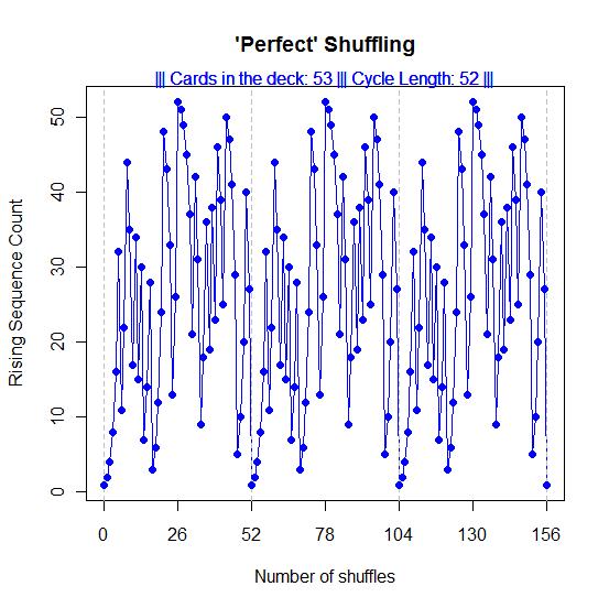
The peak and valley between shuffles 5,6, and 7 intrigued me as well. Would you have expected the RS count to rise and fall like that? Look what happens when you add one more card to the deck. It takes 52 perfect shuffles to return a 53-card deck to its starting position.





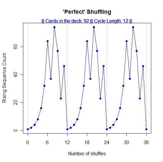
But if you add 40 cards to the deck you can get back to starting position in only 12 shuffles.





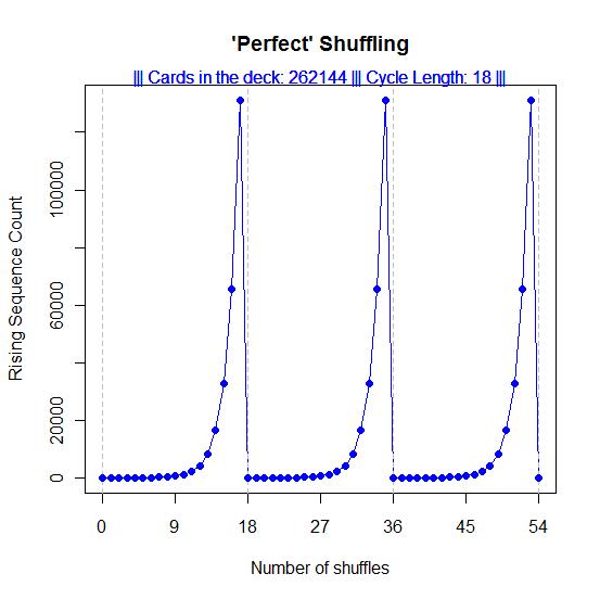
Let's consider the sequence 2ⁿ for n=1,2,3,..20.

> n=1:20
> 2**n
[1]      2      4      8     16      32
[6]     64    128    256    512    1024
[11]  2048   4096   8192  16384   32768
[16] 65536 131072 262144 524288 1048576

Decks of these sizes all return to starting position in n perfect shuffles. The program runs slow on my computer using a deck size 2¹⁸ = 262144.





Several deck sizes had interesting symmetries in their RS counts. Here is the example of a 100-card deck:

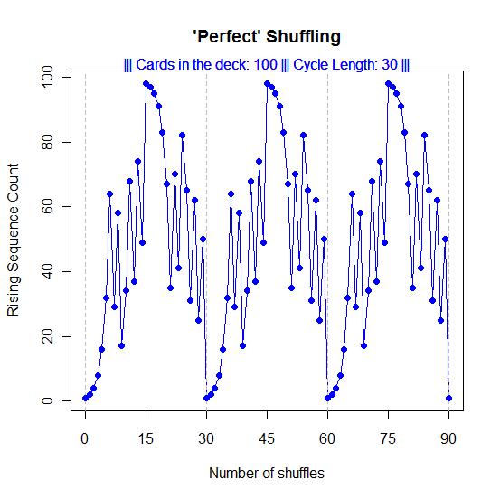It takes 30 shuffles for the 100-card deck to return to its starting position. Note that the plot is symmetric with respect to a rotation about the y=50 axis, followed by a 15-point translation on the x-axis. (Similar, but not the same, symmetry exists in the 53-card deck above, although it is harder to see at first.)


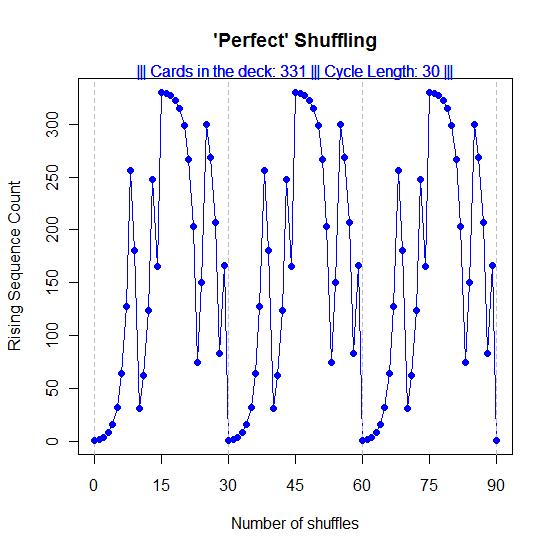
Some large prime numbers possess the rotation-translation symmetry too. Here is deck size 331:



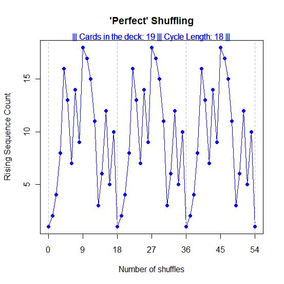
Deck size 19 is a small prime with the same symmetry, but it takes 18 shuffles to get back to start. And note how much more complicated the RS count is for 19 than the 2.7 times larger 52-card deck.





That's all I have time for right now. I'm not going to offer any explanations for the variation in RS counts as a function of deck size, let alone the various symmetries and asymmetries. I just wanted to illustrate how easy it can be find and explore some things you might not expect when using R. 


 I'll return to the shuffling topic later. 


In the meantime, you're welcome to play around with my R code yourself. You'll find a draft of it here. Copy and paste it into an R New Script window. Then, scroll down toward the bottom and look for n=52 enclosed by pound signs. Change the number 52 to anything you want, and run the code. I recommend starting with numbers less than 100,000 at first. Let me know what you find!